Last updated on November 23rd, 2025 at 05:04 am
Looking to merge two columns in Excel with a space, comma, dash or any other separator in between? This easy-to-follow guide walks you through the process step by step. Whether you’re combining first and last names or any other data, you’ll learn how to do it quickly and accurately without any hassle.
If you’re wondering how to combine two columns in Excel?, you’re in the right place! I have prepared this guide that covers multiple methods to merge data efficiently.
Suppose you have a first name in one column, and the last names are in another, and you want to merge them into one clean list, without spending hours copy-pasting.
It is a time-consuming and tedious task to copy and paste each one manually.
Here is some good news: There’s a super simple way to combine columns in Excel… and I will show you exactly how.
- How to Combine Two Columns in Excel?
- When Would You Need This?
- The Fastest Way to Combine Two Columns with a Space in Excel
- Other Ways to Combine Two Columns (If You’re Feeling Fancy)
- Practice Makes Perfect! Download Your Excel Exercise Sheet
- Quick Tips to Keep in Mind
- Pro Tips for Combining Columns in Excel
- Wrapping Up
How to Combine Two Columns in Excel?
There are several ways to merge columns in Excel, depending on your needs.
In this article, we explore different techniques like:
- & (Ampersand): = C2 & ” ” & D2
- TEXTJOIN(): =TEXTJOIN(“, “, “”, C2, D2, E2)
- CONCAT(): =CONCAT(C2, ” “, D2, ” “, E2)
- Flash Fill: Shortcut key: Ctrl + E
- VBA Macro
- Power Query
that you can use.
No stress, no fuss. This quick guide walks you through six simple ways to get it done.
When Would You Need This?
Before we dive in, here are a few common reasons you might want to combine columns:
- Creating full names from first and last names
- Joining product names with categories or codes
- Merging address fields into a single line
- Cleaning up messy data so it’s easier to read or export
Sound familiar? Cool. Let’s get into it.
The Fastest Way to Combine Two Columns with a Space in Excel
Imagine this setup:
- Column C has the first names.
- Column D has the last names. Now you want a full name in Column E, with a space in between.
One of the simplest ways to merge columns is by using the ampersand (&) operator. But is this the best method when you ask, “how to combine two columns in Excel?” Let’s find out.
Option 1: Use a Simple Formula (The & Trick) to Combine Two Columns
Steps to join columns using & (Ampersand)
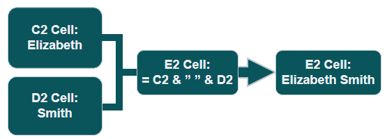
To combine two columns in Excel using Ampersand:
- Select the cell(E2 in our case) where you want to display the combined data in Excel.
- Type in this formula: = C2 & ” ” & D2

- Hit the Enter button and boom—Excel combines the two!
What’s Happening Here?
- C2 is your first column i.e. “Elizabeth”
- ” ” adds a space.
- D2 is your second column i.e. “Smith”
- When you press the Enter button, you’ll get Elizabeth Smith in E2.
Easy, right?
Now, Grab that little square (+ sign) in the bottom-right corner of the E2 cell (the fill handle) and drag it down to copy the formula to the rest of your rows.

We applied the same formula to the remaining rows.
This is the best and easiest method to combine 2 columns without losing data in Excel.
Merge using comma(,) and Dash(-)
You can use:
- = C3 & “, ” & D3 formula to combine two columns in Excel with a comma separator.

- = C2 & “- ” & D2 formula to merge using the dash in between.

Use of TEXT Function (For Formatting and Combining Numbers/Dates)
If you’re combining numbers or dates and want them formatted nicely, use TEXT() inside your formula.
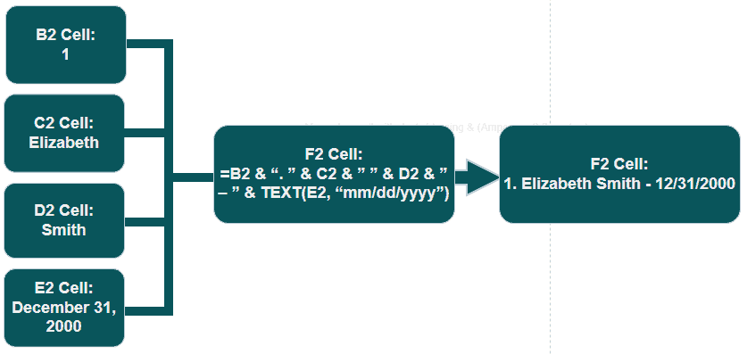
Example: =B2 & “. ” & C2 & ” ” & D2 & ” – ” & TEXT(E2, “mm/dd/yyyy”)

Here you can see that Colum B has a number and E has a date. We applied the TEXT() function to join all four column values in the F column.
Tips: If you want to combine more than two columns i.e. B2, C2, and D2, You can use the formula = B2 & ” ” & C2 & ” ” & D2
Related Excel Guide
- Compare Two Columns in Excel
- Remove Duplicates in Excel
- Combine Date and Time in Excel
- Combine Multiple Columns in Excel Using VBA
- Record a Macro for Find and Replace in Excel
- Replace Words in Excel
- Split Text into Columns in Excel
- Separate Date and Time in Excel
Other Ways to Combine Two Columns (If You’re Feeling Fancy)
Here are other options which you can use to combine two or more columns of data.
Option 2: Use TEXTJOIN()
This function is perfect for working with more than two columns or for ignoring blank cells.
Suppose you have a scenario in which a First name is in column C, a Last name is in Column D, an Address is in column E, and a few cells are empty. You want to combine multiple columns in column F.
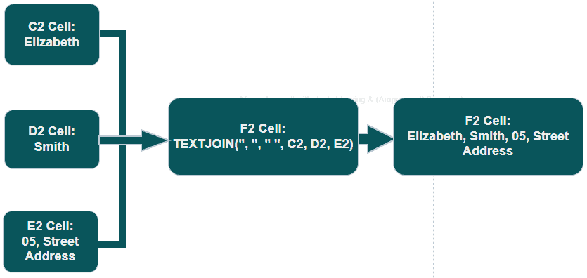
Steps to join cells using the TEXTJOIN() function in Excel.
- Select cell F2.
- Type in formula =TEXTJOIN(“, “, “”, C2, D2, E2)
- Hit Enter.

What’s Happening Here?
- The ” ” part is your separator (in this case, a space). You can use commas or dashs as a separator if you need.
- TRUE skips any blanks.
In the above image, you can see that we have used the TEXTJOIN function to merge data from C, D, and E columns into F.
Quick Tip: If you type =TEXTJOIN in a cell and it shows a #NAME? error, your Excel (Excel 2016 or earlier versions) version probably doesn’t support it. This function was introduced in Excel 2019 and is available in Excel 365 (Microsoft 365), Excel 2019 for Windows and Mac, and Excel Online (browser version).
Option 3: Use CONCAT() (For Newer Versions of Excel)
If you’ve got Excel 2019 or newer, you can try the CONCAT() function. This is basically an upgrade from CONCATENATE().
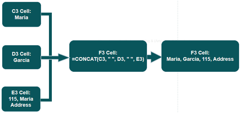
We will use the same example as described in option 2 to join three columns.
A step-by-step guide for joining cells in Excel using the Concat() function.
- Step 1: Click on cell F2.
- Step 2: Write formula =CONCAT(C2, ” “, D2, ” “, E2)
- Step 3: Press the Enter key on the keyboard.

You can use the CONCAT() or CONCATENATE() function and the other six methods to combine date and time in Excel.
Why CONCAT() instead of CONCATENATE()
Starting with Excel 2016, Microsoft introduced the CONCAT() function as a more powerful and flexible replacement for CONCATENATE().
Key points:
- CONCATENATE() is still available in Excel 2016 and later versions for backward compatibility, but it’s considered deprecated.
- Microsoft recommends using CONCAT() or TEXTJOIN() (introduced in Excel 2016) going forward.
Opposite of Concatenation in Excel: How to Split Text Using Shortcut, Formula, and Function
- Antonym of Concatenation: The opposite of combining text is splitting it into multiple columns or cells.
- Shortcut for Splitting Text: Use the Text to Columns shortcut (Alt + A + E) to separate text based on a delimiter like commas or spaces.
- How to Do It with a Formula: Use LEFT(), RIGHT(), and MID() functions to extract specific parts of text.
- VBA Function for Splitting: The Split() function in Excel VBA divides a string into an array based on a delimiter.
- TEXTSPLIT() Function: A dynamic formula in Excel 365 that automatically separates text into multiple cells.
Here is a detailed guide on splitting Text into Columns using all above mentioned formulas and functions.
Option 4: Flash Fill (The Lazy Person’s Hack!)
Flash Fill is Excel’s auto-magic tool that detects patterns and fills in the rest for you. No formula is required!
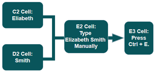
How to use Flash Fill to join cells:
- In E2, manually type Elizabeth Smith as per our example.
- Press the Enter button. The cursor will move on E3
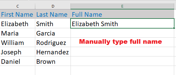
- Start typing the next combined value in E3, like: Maria. Or Ctrl + E Shortcut.

- Excel will recognize the pattern and show flash-fill suggestions.
- Press the Enter button. Boom! The remaining cells will be filled automatically with the same pattern.

This is the perfect option for quick-and-dirty tasks, no formulas left behind!
Option 5: Combine Two Columns Using VBA Macro
Scenario:
You have First Names in Column C and Last Names in Column D, and you want to combine them into Column E, separated by a space.
Steps:
Here is a step-by-step guide to join 2 columns in Excel using a Macro.

Step 1: Open Your Excel Workbook
Make sure your workbook has the data in the C and D columns
For example:

Step 2: Access the VBA Editor
- Press Alt + F11 on your keyboard.
- This opens the VBA Editor window.
- In the editor, click Insert > Module.
- A new blank code window will appear where you can write your macro.

Step 3: Paste the VBA Code
Here’s a simple macro to amalgamate columns C and D into column E:
Sub CombineColumns()
    Dim ws As Worksheet
    Dim lastRow As Long
    Dim i As Long

    'Set your worksheet (ActiveSheet means the sheet you're currently on)
    Set ws = ActiveSheet

    'Find the last row with data in column C
    lastRow = ws.Cells(ws.Rows.Count, "C").End(xlUp).Row

    'Loop through each row to combine data
    For i = 2 To lastRow
        ws.Range("E" & i).Value = ws.Range("C" & i).Value & " " & ws.Range("D" & i).Value
    Next i

    MsgBox "Columns Combined Successfully!", vbInformation
End SubStep 4: Close the VBA Editor
- Click the X to close the editor.
- Go back to your Excel sheet.
Step 5: Run the Macro
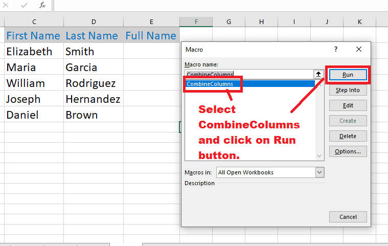
- Press Alt + F8
- This opens the “Macro” dialog box.
- Select CombineColumns from the list.
- Click Run.
What Happens?
The macro loops through each row of your data (starting from row 2), combines the First Name and Last Name from columns C and D, and places the full name in column E.
For example:
- C2 = Elizabeth
- D2 = Smith
- E2 becomes Elizabeth Smith
Breakdown of the VBA Code
- Dim ws As Worksheet: Declares a worksheet variable.
- Set ws = ActiveSheet: Sets the active sheet as your working sheet.
- lastRow = ws.Cells(…).End(xlUp)…: Finds the last row in column C with data.
- For i = 2 To lastRow: Loops from row 2 to the last row.
- ws.Range(“E” & i).Value = …: Combines the values and writes to column E.
- MsgBox: Pops up a message when it’s done.
Bonus: Add a Button to Run the Macro (Optional, But Fun!)
Want to click a button instead of pressing Alt + F8 every time?
Here’s how:
- Go to the Developer tab. (If you don’t see it, go to File > Options > Customize Ribbon > Check Developer and click OK.)
- Click Insert > Button (Form Control).
- Draw your button anywhere on your sheet.
- When prompted, assign your macro (CombineColumns) to it.
- Right-click the button to edit the text (call it “Combine Names” or whatever you like).
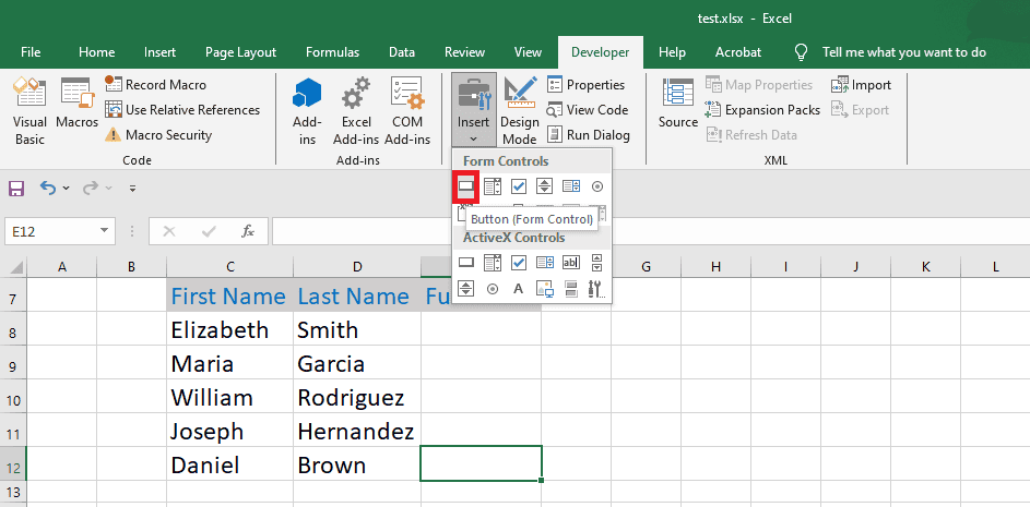

Now just click your button, and the macro will run automatically!
Option 6: Merge Using Power Query (Step-by-Step)
If you’re working with large datasets and looking for a more automated solution, Power Query is a powerful tool. You can easily join columns without writing any formulas.
Here’s how you can do it:
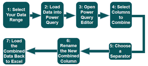
Step 1: Select Your Data Range
First, select the two columns that contain the data you want to merge in Excel.
Example:
| First Name | Last Name |
| Elizabeth | Smith |
| Maria | Garcia |
| William | Rodriguez |
| Joseph | Hernandez |
| Daniel | Brown |
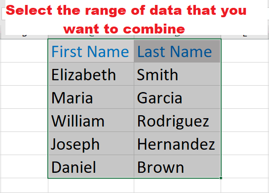
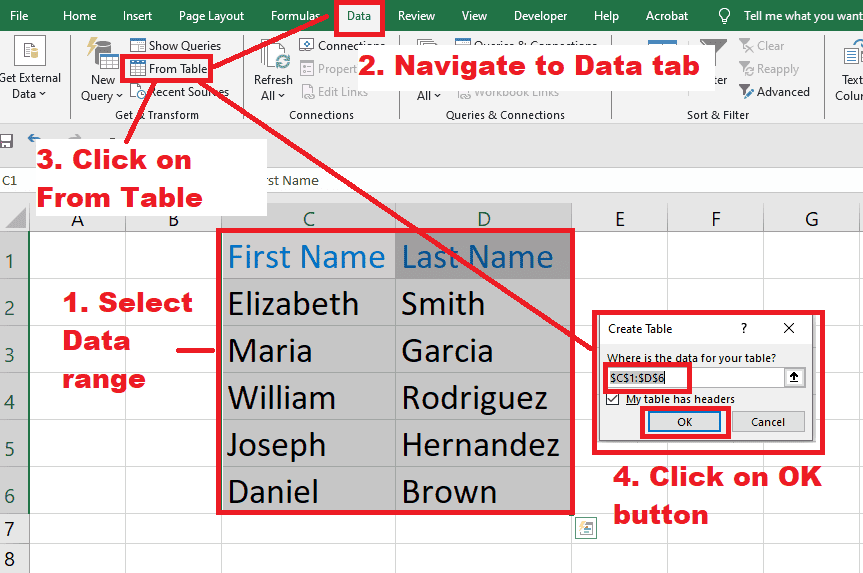
Step 2: Load Data into Power Query
- Go to the Data tab on the Excel ribbon.
- Click From Table/Range. It will ask to create a table.
- Click on the OK button.
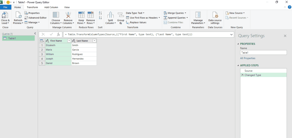
Step 3: Open Power Query Editor
Your data will open in the Power Query Editor window.
Step 4: Select Columns to Combine
Hold Ctrl and select both columns you want to combine (e.g., First Name and Last Name).

Navigate to the Transform tab at the top.
Click Merge Columns.

Step 5: Choose a Separator
A dialog box will pop up asking you to select a separator:
You can choose Space, Comma, Colon, Equals Sign, Semicolon, Tab, or type a Custom Separator.
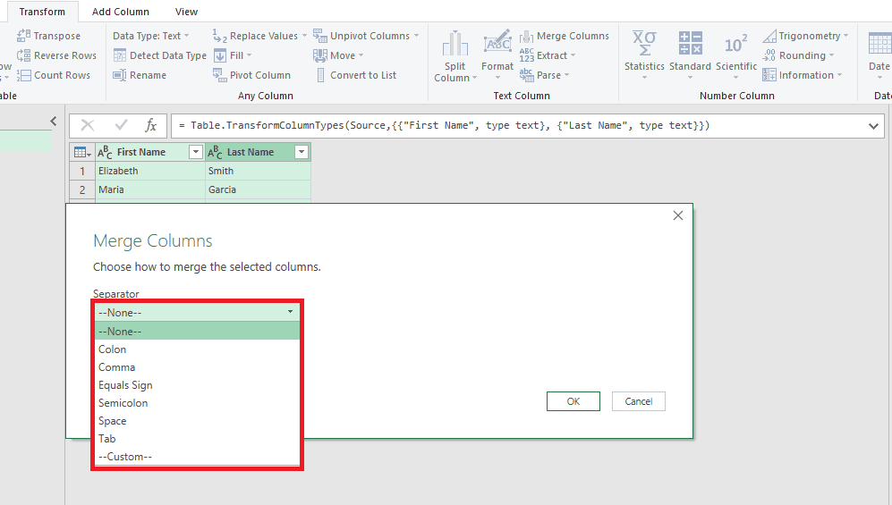
Example: Select Space to combine Elizabeth and Smith into Elizabeth Smith.
Step 6: Rename the New Combined Column
After merging, Power Query creates a new column called Merged by default.
Rename it to Full Name.
Click on the OK button.

Both columns will combine in the Power Query editor.
Step 7: Load the Combined Data Back to Excel
Go to the Home tab in Power Query.
Click Close & Load.

The united data will appear in a new worksheet or table in Excel.

That’s it. Your data is merged in a single column using the Power Query editor.
Why Use Power Query?
Here are a few important reasons for using Power Query.
- No formulas to manage.
- Great for large data sets and repeatable tasks.
- You can automate updates when your source data changes—just refresh!
Pro Tip while using Power Query:
If you need to split the combined column later, Power Query has a Split Column option too!
Practice Makes Perfect! Download Your Excel Exercise Sheet
Learning how to combine columns in Excel is one thing… but practicing it? That’s where the real magic happens.
I’ve put together an exercise sheet just for you! Inside, you’ll find ready-made data to practice:
- Simple & formulas (&, TEXT Function)
- TEXTJOIN() and CONCAT() methods
- Flash Fill tricks
- Even a spot to run your first VBA macro!
Click below to download your practice workbook (it’s free!):
Download the Excel Exercise Sheet Now!
(It’s a .xlsx file, totally safe, and won’t ask for your email.)
What’s Inside the Exercise Sheet?
Here’s a sneak peek of what you’ll get:
- First Names and Last Names in Columns C and D to practice combining into Column E
- Tasks for:
- Combining columns with a space, comma, or dash.
- Ignoring blank cells using TEXTJOIN()
- Creating full names with prefixes/suffixes
- Running a simple VBA macro to automate the process
- A step-by-step guide right in the sheet so you won’t get lost!
How to Use It
- Download the file and open it in Excel.
- Start with Sheet 1, where you’ll practice basic formulas.
- Move to the Advanced Methods sheet for TEXTJOIN(), CONCAT(), and VBA.
- Challenge yourself by solving the Bonus Tasks I’ve included!
Why Practice With This Sheet?
- It’s hands-on, not just theory
- You can see the formulas in action
- Perfect if you want to learn by doing
- Helps build muscle memory, so combining columns becomes second nature!
Quick Tips to Keep in Mind
- Customize your separator: Use a comma, hyphen, dash, or anything else. Just replace the ” ” with whatever you need.
- Lock the combined values: If you want to get rid of formulas, copy Column E, then right-click and choose Paste Values.
- Works with numbers too: Combine product codes, IDs, anything.
Combining columns in Excel seems simple, but sometimes you might run into issues like #VALUE! errors, wrong formatting, or data loss.
Check out this detailed guide on Fixing Common Errors When Combining Columns in Excel to troubleshoot and fix these problems quickly!
Pro Tips for Combining Columns in Excel
Combining columns can be simple, but a few smart tricks can make your work cleaner and more efficient. Here are some pro tips to level up your Excel skills:
1. Avoid Extra Spaces with the TRIM() Function
When you combine columns, sometimes there are unwanted leading or trailing spaces in your data, especially if the source data isn’t clean. This can make your combined data look messy.
How to Fix It:
You can wrap each cell reference inside the TRIM() function to remove extra leading and trailing spaces.
Here is an example:
=TRIM(C2) & " " & TRIM(D2)
In the above image, you can see that the TRIM() function has removed leading and trailing space and combined results neat and free from space.
2. Handle Empty Cells Gracefully
If you combine columns and one of them is blank, you may end up with unnecessary spaces or delimiters.
How to Fix It:
Use the IF() function to check if a cell is empty before adding spaces or punctuation.
Example for clarity:
=C2 & IF(D2<>"", " - " & D2, "")
3. Use CHAR Functions for Line Breaks
Are you looking to split combined data across multiple lines in one cell?
You can insert line breaks using CHAR(10) and enable Wrap Text.
How to Do It:
Here is a formula with an example
=C2 & CHAR(10) & D2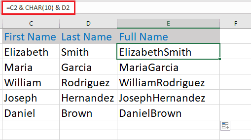
After entering the formula, go to the Home tab → Wrap Text to make it display properly.
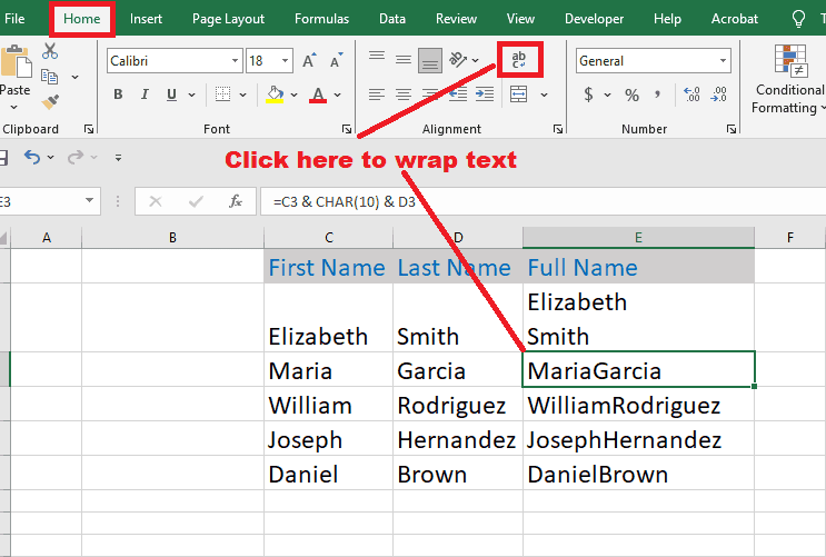
This is very useful when you are combining long texts like addresses, descriptions, etc.
4. Convert Formulas to Static Text (Values Only)
Now you have a complete idea about how to merge two columns in Excel without losing data using different formulas and methods. But what if you want to remove the formulas and keep only the values?
I have a solution for you.
How to Do It:
Here are the steps to do it.
Steps:
Step 1: Copy the combined column (Ctrl + C).
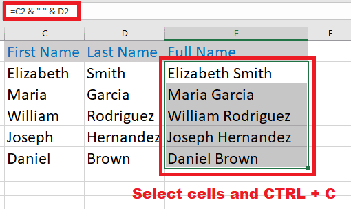
Step 2: Right-click → Paste Special → Values.

Now you have plain text instead of formulas! Easy!
FAQs on Combining Two Columns in Excel
How can I combine two columns without losing data in Excel?
You can use the & operator or the TEXTJOIN() function. These methods preserve your original data and return the combined result in a new column. Earlier in this article, we have explained both methods with examples.
What is the shortcut to combine cells in Excel?
Flash Fill (Ctrl + E) is the fastest way to combine columns without using formulas. It’s available in Excel 2013 and later versions.
Can I combine columns in Excel with a space or comma?
Yes, you can! Use the formula =A1 & " " & B1 to add a space between values, or =A1 & ", " & B1 to separate them with a comma.
How do I combine columns in Excel without formulas?
You can use Flash Fill (Ctrl + E) to automatically combine patterns without writing formulas. Simply start typing the combined result in a new column, and Excel will detect and fill the rest.
How to combine two columns into one without losing formatting?
To preserve formatting while combining columns, use TEXT() within your formula. For example: =TEXT(A1,"mm/dd/yyyy") & " - " & B1.
Wrapping Up
Now that you’ve learned different ways to merge columns, which method works best for you? Try them out and let us know! Still unsure how to combine two columns in Excel? Drop a comment below!